Linearity of Expectation

In this note, we will introduce linearity of expectation for discrete random variables, how it’s used, why it’s useful, and very important subtleties. Along the way, we’ll prove a few useful things you might see in computer science.

We will assume you possess basic knowledge on what a discrete random variable is. Nothing formal here, we won’t be fully using the axiomatic method here but we’ll at least give a little formalism here because it will be useful to see things in this new light. Just bear in mind we won’t be going 100% formal, but just a taster of how to be a little more well-founded in what we do.

Introduction

You should think random variable $X$ as a variable that takes on potentially more than one value (it could also be just one value but that’s not very random nor interesting, is it?).

So $X$ has a set of values $E$ that it can take on, think of this as the set of possible events $E$. Furthermore, for each value $e\in E$, we want to associate with it a value $p_e$. You can now see this as a function $P:e\to \mathbb{R}$. There are a few more requirements about these values.

1. $P(e)\ge 0$, $\forall e\in E$.
2. ${\sum }_{e\in E}P(e)=1$

In fact, we use $\mathrm{Pr}[X=e]$ as notation for $P(e)$.

Did you notice we basically just called it a function? Here’s the idea, we have some kind of phenomenon in real life we wish to model, but there’s some degree of uncertainty we have about that phenomenon. For example, something like “Which face of a dice will be on the top?” after we roll it. We would like to assign each outcome $1,2,3,4,5,6$ individually with a number in $\mathbb{R}$. What kind of number? Well it has to satisfy the constraints laid out above. For example, if we know the dice is “fair”, to model that dice using our mathematical objects we would say $\mathrm{Pr}[X=i]=\frac{1}{6},\forall i\in \{1,2,3,4,5,6\}$. If the dice was loaded and unfair instead we might assign different values to each outcome.

Note

Now to be clear these are not axioms of probability, rather, these requirements actually follow from the actual axioms of probability which I will not show because it is rather complicated. But you may treat this as the foundation on which we will start. Like how it might feel to learn Python instead of C, where the low-level details have been done for you, and you’re here to think about higher level details.

Anyway, there’s always the abstract question of “what does it mean for a phenomenon to have some probability?“. There’s the whole Frequentist vs Bayesian debate (that’s a whole big can of worms). So I just want you to appreciate the fact that at a very abstract level: we are just assigning numbers from our set of events $E$ to real values that satisfy the constraints that I mentioned.

Now technically speaking, there’s one more thing I should mention: A random variable is not the same as its distribution. A distribution is basically the function $P:E\to \mathbb{R}$ that satisfies the properties I mentioned. A random variable needs to take a distribution. Think of a variable as an instance. You could have two random variables $X_1,X_2$ that are identically distributed (they have the same function $P$ but potentially different outcomes). We will say two random variables are identically distributed if they have the same distribution function $P$.

For example, if we had 2 perfect copies of the same fair, perfect, independent coin, then we could say there’s two random variables $C_1,C_2$ that both have the same distribution where $\mathrm{Pr}[C_1=head]=\mathrm{Pr}[C_1=tail]=\frac{1}{2}$.

Lastly, we will call a random variable discrete, if the event set $E$ is discrete.

Expected Value of a Random Variable

So given a discrete random variable $X$, one thing we might want to ask is “What is the expected value?“. We will use $\mathbb{E}[X]$ to denote this value. First of all, the interesting thing about the expected value is that we can prove (as a separate theorem) that if we took $n$ trials of measuring $X$, you can think of this as $X_1,X_2,X_3,\dots ,X_n$ where they are all identically distributed as $X$ and all fully independent of each other, and we measured the value $\frac{{\sum }_{i=1}^t{X}_i}{n}$ then this will converge to $\mathbb{E}[X]$ as $n\to \infty$. So here, we care about random variables $X$ that take on values in $\mathbb{R}$. i.e. the event set of $X$ are values we can add and divide.

Does this mean $X$ is most likely to take on value $\mathbb{E}[X]$? No. But nonetheless it tells us that if we are happy with many trials of $X$, the “average value” that we will see, should be close to $\mathbb{E}[X]$.

The definition of the expectation of a random variable $X$ is given as:

$$\mathbb{E}[X]=\sum _{a\in E}a\cdot \mathrm{Pr}[X=a]$$

Now, there are other possible and equivalent formulations (shown as theorems) but we’ll stick with this one. Also, perhaps it’s pretty intuitive why this is the right definition. For example, we expect to see value $a$, about $\mathrm{Pr}[X=a]$ fraction of the time.

So for example, if we let a coin $C$ be such that $Pr[C=1]=p$, and $Pr[C=0]=1-p$, then the expected value $\mathbb{E}[C]=1\cdot p+0\cdot (1-p)=p$.

As another example, a dice $D$ with uniform probability of taking values $1,2,3,4,5,6$ will yield $\mathbb{E}[D]={\sum }_{i=1}^6\frac{i}{6}=\frac{6(7)}{2}\cdot \frac{1}{6}=\frac{21}{6}$.

Conditioning Random Variables

Now if all we had to study was single random variables, this would not be so interesting. Let’s consider the following scenario: We have a bag that has 5 balls with the following values: $1,2,2,8,8$.

And we want to draw two balls without replacement, and output their values. There’s two ways we model this:

Method 1: Directly creating a single random variable.

One way is to make a single random variable $B$ that takes on $1$ of $5$ possible values: $3,4,9,10,16$, like so:

1. $\mathrm{Pr}[B=3]=\frac{1\times 2+2\times 1}{5\times 4}=\frac{4}{20}=\frac{1}{5}$. Either take the $1$-ball first, then either of the $2$-balls, or the other way around.
2. $\mathrm{Pr}[B=4]=\frac{2\times 1}{5\times 4}=\frac{1}{10}$. You have to take both of the $2$-balls.
3. $\mathrm{Pr}[B=9]=\frac{1\times 2+2\times 1}{5\times 4}=\frac{4}{20}=\frac{1}{5}$. Either take the $1$-ball first, then either of the $8$-balls, or the other way around.
4. $\mathrm{Pr}[B=10]=\frac{2\times 2+2\times 2}{5\times 4}=\frac{8}{20}=\frac{2}{5}$. Either take one of the $2$-balls first, then either of the $8$-balls, or the other way around.
5. $\mathrm{Pr}[B=16]=\frac{2\times 1}{5\times 4}=\frac{1}{10}$. You have to take both of the $8$-balls.

Then from this you can also do stuff like find $\mathbb{E}[B]$.

Method 2: Creating two random variables instead.

We can instead create two random variables $B_1$ that models the first draw, and $B_2$ that models the second. However, there are very important subtleties that crop up in linearity of expectation later on, so pay some attention here.

$B_1$’s distribution looks like this:

1. $\mathrm{Pr}[B_1=1]=\frac{1}{5}$
2. $\mathrm{Pr}[B_1=2]=\frac{2}{5}$
3. $\mathrm{Pr}[B_1=8]=\frac{2}{5}$

But what about $B_2$? To be clear we cannot just say that $B_2$‘s distribution is the same as $B_1$. In some sense, because $B_2$‘s outcome depends on $B_1$. To be clear, we want to figure out what $\mathrm{Pr}[B_2=1],\mathrm{Pr}[B_2=2],\mathrm{Pr}[B_2=8]$ are.

Now, $\mathrm{Pr}[B_2=1]=\mathrm{Pr}[B_1=1\cap B_2=1]+\mathrm{Pr}[B_1=2\cap B_2=1]+\mathrm{Pr}[B_1=8\cap B_2=1]$. Think of this as saying: The probability that $B_2$ takes value $1$ is the sum of the probability of all the possible cases of what $B_1$ takes.

If that is not so convincing, you can think of it the following way:

$$\begin{array}{rl}\mathrm{Pr}[B_2=1]=& \mathrm{Pr}[B_2=1|B_1=1]\cdot \mathrm{Pr}[B_1=1]\\ & +\mathrm{Pr}[B_2=1|B_1=2]\cdot \mathrm{Pr}[B_1=2]\\ & +\mathrm{Pr}[B_2=1|B_1=8]\cdot \mathrm{Pr}[B_1=8]\end{array}$$

Which is to say, either $B_1$ is $1$ with some probability, then conditioned on that probability, $B_2$ takes $1$ with some probability (accounting for the fact that the first ball drawn was $1$). So filling in these values, we get it to be:

$$\begin{array}{rl}\mathrm{Pr}[B_2=1]=& 0\cdot 1+\frac{1}{4}\cdot \frac{2}{5}+\frac{1}{4}\cdot \frac{2}{5}\\ =& \frac{4}{4\times 5}\\ =& \frac{1}{5}\end{array}$$

Now isn’t that curious? Somehow it’s the same value. Indeed if you worked this out for $\mathrm{Pr}[B_2=2],\mathrm{Pr}[B_2=8]$, you get:

$$\begin{array}{rl}\mathrm{Pr}[B_2=2]=& \mathrm{Pr}[B_2=2|B_1=1]\cdot \mathrm{Pr}[B_1=1]\\ & +\mathrm{Pr}[B_2=2|B_1=2]\cdot \mathrm{Pr}[B_1=2]\\ & +\mathrm{Pr}[B_2=2|B_1=8]\cdot \mathrm{Pr}[B_1=8]\\ =& \frac{2}{4}\cdot \frac{1}{5}\\ & +\frac{1}{4}\cdot \frac{2}{5}\\ & +\frac{2}{4}\cdot \frac{2}{5}\\ =& \frac{2}{20}+\frac{2}{20}+\frac{4}{20}=\frac{8}{20}=\frac{2}{5}\end{array}$$

Also, $\mathrm{Pr}[B_2=8]$ works in similar way. Crazy isn’t it? Why is $B_2$ identically distributed to $B_1$?

Question

What? I don’t get it. Why does $B_2$ look like this? Okay, I need you to think in the following way: We drew two balls without replacement, let’s call it $b_1$, $b_2$. But then we threw the first ball $b_1$ away and only looked at the second ball $b_2$. It’s a little trippy but this actually has the same distribution if we drew two balls without replacement, and then threw away the second ball $b_2$ and only looked at the first ball $b_1$.

In general for any distribution here’s the idea (let’s just do it for 2 draws without replacement): Let $S$ be a set of items $\{s_1,s_2,\dots ,s_n\}$, with frequencies $freq:S\to {\mathbb{Z}}^{+}$. Let $T={\sum }_{s\in S}freq(s)$. $T$ is basically the total number of items.

For example, with balls $1,2,2,8,8$, then $S=\{1,2,8\}$, and $freq(1)=1$, $freq(2)=2$, and $freq(8)=2$. Then $T=5$.

Okay we first think to note: Let $X_1$ be the first draw from the set $S$ based on their frequencies. Then $\mathrm{Pr}[X=i]=\frac{freq(i)}{T}$. Let’s consider sets $S$ where $T\ge 2$. I.e. There are at least $2$ items to draw or else we cannot make a second draw in the first place.

The question is what is $X_2$. So in general:

$$\begin{array}{rl}\mathrm{Pr}[X_2=i]& =\sum _{s\in S}\mathrm{Pr}[X_2=i|X_1=s]\cdot \mathrm{Pr}[X_1=s]\\ & =\mathrm{Pr}[X_2=i|X_1=i]\cdot \mathrm{Pr}[X_1=i]+\sum _{s\in S,s\ne i}\mathrm{Pr}[X_2=i|X_1=s]\cdot \mathrm{Pr}[X_1=s]\\ & =\frac{freq(i)-1}{T-1}\cdot \frac{freq(i)}{T}+\sum _{s\in S,s\ne i}\frac{freq(i)}{T-1}\cdot \frac{freq(s)}{T}\\ & =\frac{freq(i)-1}{T-1}\cdot \frac{freq(i)}{T}+\frac{freq(i)}{(T-1)T}\sum _{s\in S,s\ne i}freq(s)\\ & =\frac{freq(i)-1}{T-1}\cdot \frac{freq(i)}{T}+\frac{freq(i)}{(T-1)T}(T-freq(i))\\ & =\frac{freq(i)}{T(T-1)}(freq(i)-1+(T-freq(i)\left)\right)\\ & =\frac{freq(i)}{T(T-1)}(T-1)\\ & =\frac{freq(i)}{T}\end{array}$$

That looks suspiciously like $\mathrm{Pr}[X_1=1]$ innit?

Explanation

Line 1 follows from Bayes’ theorem.

Line 2 from splitting the sum based on whether $s=i$ or not. We need to treat them differently.

Line 3 follows from the fact that given $X_1=i$, there are $freq(i)-1$ copies of $i$ remaining, and the total is reduced down to $T-1$.

Line 3 also follows from the fact that given $X_1=i$ where $i\ne s$, there are still $freq(i)-1$ copies of $i$ remaining, and the total is reduced down to $T-1$.

Line 4 just factors out the portions independent of $s$.

Line 5 follows from the fact we’re adding up all the frequencies except $freq(i)$ so this is just the total without $freq(i)$, or $T-freq(i)$.

Line 6 onwards is just basic algebra.

Now to be very clear: $B_1$ and $B_2$ are not independent. Why? $\mathrm{Pr}[B_1=1\cap B_2=1]=0$ but $\mathrm{Pr}[B_1=1]\cdot \mathrm{Pr}[B_2=1]=\frac{1}{25}$. So $\mathrm{Pr}[B_1=1\cap B_2=1]\ne \mathrm{Pr}[B_1=1]\cdot \mathrm{Pr}[B_2=1]$, which is enough to argue that $B_1$ and $B_2$ are not independent.

Linearity of Expectation

Okay, given what we know from the previous section, we can now ask the following question: What is the expected value of the sum of the values of the two balls drawn? Well if you used method 1 from above, then you’d just have to do $3\times \frac{1}{5}+4\times \frac{1}{10}+9\times \frac{1}{5}+10\times \frac{2}{5}+16\times \frac{1}{10}$.

Or you could use method 2, and now you know that $B_1$ and $B_2$ are identically distributed, so you really just need to find $\mathbb{E}[B_1]$. This happens to be a lot simpler: $1\times \frac{1}{5}+2\times \frac{2}{5}+8\times \frac{2}{5}$. Then, if we believe in linearity of expectations, we know that

$$\mathbb{E}[B_1+B_2]=\mathbb{E}[B_1]+\mathbb{E}[B_2]=2\times \mathbb{E}[B_1]=2\times \left(1\times \frac{1}{5}+2\times \frac{2}{5}+8\times \frac{2}{5}\right)$$

What if the two draws were with replacement?

Well then I hope you know that definitely $B_1$ and $B_2$ are identically distributed. And furthermore, if the draws were with replacement (and both draws were done the same way), then $B_1$ and $B_2$ are independent. So the above equation still holds!

Proof of Linearity of Expectation

Again, we want to show something like given two random variables $X,Y$, that may or may not be independent, $\mathbb{E}[X+Y]=\mathbb{E}[X]=\mathbb{E}[Y]$.

So why does it not matter if two variables are independent or not? Let’s see:

$$\mathbb{E}[X+Y]=\sum _a\sum _b(a+b)\mathrm{Pr}[X=a,Y=b]$$

Now because $X,Y$ are not necessarily independent, we cannot write $Pr[X=a,Y=b]=\mathrm{Pr}[X=a]\cdot \mathrm{Pr}[Y=b]$. However, let me split the sum into two summations first.

$$\begin{array}{rl}\mathbb{E}[X+Y]& =\sum _a\sum _b(a+b)\mathrm{Pr}[X=a,Y=b]\\ & =\sum _a\sum _{b}a\cdot \mathrm{Pr}[X=a,Y=b]+\sum _a\sum _{b}b\cdot \mathrm{Pr}[X=a,Y=b]\\ & =\sum _{a}a\cdot \sum _b\mathrm{Pr}[X=a,Y=b]+\sum _{b}b\cdot \sum _a\mathrm{Pr}[X=a,Y=b]\end{array}$$

Now there’s two parts we need to handle, but they’re handled with the same idea: If we fix $a$, and said $X=a$, then summing across all $\mathrm{Pr}[X=a,Y=b]$, where we vary the value $b$, then the value is actually just $\mathrm{Pr}[X=a]$. Think of it this way, $\mathrm{Pr}[X=a]$ can be broken up into disjoint parts $\mathrm{Pr}[X=a,Y=1],\mathrm{Pr}[X=a,Y=2],\mathrm{Pr}[X=a,Y=3],\dots$ and so on. If we added them all back up, we just get $\mathrm{Pr}[X=a]$ again. Below is an example of this intuition with $Y$ taking on $7$ possible values:

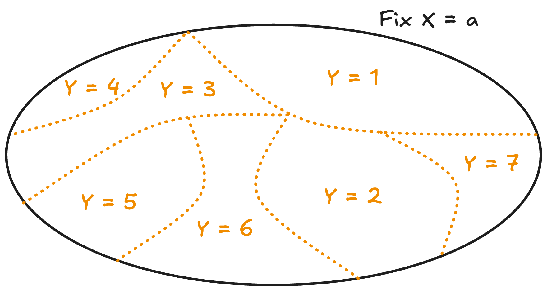
So because of that:

$$\sum _{a}a\cdot \sum _b\mathrm{Pr}[X=a,Y=b]=\sum _{a}a\mathrm{Pr}[X=a]=\mathbb{E}[X]$$

and likewise:

$$\sum _{b}b\cdot \sum _a\mathrm{Pr}[X=a,Y=b]=\sum _{b}b\mathrm{Pr}[Y=b]==\mathbb{E}[X]$$

which means the original two parts just becomes $\mathbb{E}[X]+\mathbb{E}[Y]$.

Where do we use Linearity of Expectations in CS?

Many places! I will show you a few things that you might see in CS2040S, and CS3230.

The Classic Hat Check Problem

Let’s say there are $n$ people, each person has a unique label from $\{1,2,\dots ,n\}$. They each also have a unique hat. The $i^{th}$ person basically has the $i^{th}$ hat. They enter the restaurant to dine, and as they leave, they each take a remaining hat uniformly at random. Effectively, you can also think of this as the $n$ hats being permuted uniformly at random. I.e. put a random permutation function $\pi :\{1,2,\dots ,n\}\to \{1,2,\dots ,n\}$. Then the $i^{th}$ person gets the $\pi (i{)}^{th}$ hat.

How many people do we expect to get their hat back? Going through $n$ permutations is a big pain if you want to do the following:

$$\sum _{i=0}^{n}i\cdot \mathrm{Pr}[X=i]$$

In particular, if we let $X$ be the random variable that counts how many people get their hat back, to get $\mathrm{Pr}[X=i]$ you’d effectively kind of have to use generalised principle of inclusion exclusion.

There’s a slightly easier way if you know that since $X$ takes on value in $\mathbb{N}$ we can also use:

$$\mathbb{E}[X]=\sum _{i=0}^{\infty }\mathrm{Pr}[X\ge i]$$

and this makes the task slightly easier, but still a little tricky because you’ll have a lot of factorials that you’ll need to simplify.

So here’s the simplest possible way (a technique you’ll see again in the future):

Let $X_i$ be a random variable that is $1$ if $\pi (i)=i$, and $0$ otherwise. So think of $X_i$ as basically adding to a counter when it’s happy (i.e. when the $i^{th}$ person gets their hat back).

Now to be clear, between any $i,j$, $X_i$ and $X_j$ are definitely correlated. After all, you’d expect $X_j$ to be more likely to be $1$ when $X_i$ is also $1$. The probability of the outcomes of $X_j$ change when we know what $X_i$ is. That said, there’s nothing wrong with writing:

$$X=\sum _{i=1}^n{X}_i$$

Now $X$ literally counts the number of people who got their hat back. E.g. when all $X_i$ are $0$, no one got their hat back, so $X=0$. So now what is $\mathbb{E}[X]$? Well that’s just:

$$\mathbb{E}\left[X\right]=\mathbb{E}\left[\sum _{i=1}^n{X}_i\right]=\sum _{i=1}^n\mathbb{E}[X_i]$$

So why’s this so significant? Because it tells us that instead of worrying about the correlations, we can get the expected values separately. Which is a huge load of work off our shoulders. Indeed, fix any $i$, let’s look at what happens:

$$E[X_i]=1\cdot \mathrm{Pr}[X_i=1]+0\cdot \mathrm{Pr}[X_i=0]$$

Which means that the expected value of $X_i$ is just the probability that it is $1$.

So what is the probability that it is $1$? Well, there are $(n)!$ permutations, and there are $(n-1)!$ many permutations where we insist that $\pi (i)=i$. So the probability is $\frac{(n-1)!}{n!}=\frac{1}{n}$. So coming back to our original working:

$$\mathbb{E}\left[X\right]=\mathbb{E}\left[\sum _{i=1}^n{X}_i\right]=\sum _{i=1}^n\mathbb{E}[X_i]=\sum _{i=1}^n\frac{1}{n}=1$$

So regardless of the number of people, in expectation only $1$ person will get their hat back.

Quicksort analysis

So you’ve probably learned quicksort by now. As a quick refresher, let’s see the algorithm again:

function quicksort(xs) {
    // Let k = length of xs
    // O(1)
    if (is_null(xs) || is_null(tail(xs))) {
        return xs;
    } else {
        // O(k)
        const pivot_index = math_floor(math_random() * length(xs));
        // let i = value of pivot_index
        // O(i)
        const pivot = list_ref(xs, pivot_index);
 
        // O(k)
        const lower = filter(x => x < pivot, xs);
        // let l = length of lower
        // O(k)
        const pivots = filter(x => x === pivot, xs);
        // let p = length of pivots
        // O(k)
        const higher = filter(x => x > pivot, xs);
        // let h = length of higher
 
        // T(l)
        const sorted_lower = quicksort(lower);
        // T(h)
        const sorted_higher = quicksort(higher);
 
        // O(p + h)
        return append(append(sorted_lower, pivots), sorted_higher);
    }
}

Now you might have been taught that this runs in $O(n^2)$ time because in the worst case, the array might because the every time we recurse the list might only be of size $1$ smaller or something along those lines.

But what if we always randomly picked a pivot to use in the partitioning step? What happens then?

We can actually show the expected runtime is $O(n\log n)$. You can imagine how using:

$$\mathbb{E}[X]=\sum _{i=0}^{\infty }i\cdot \mathrm{Pr}[X=i]$$

would be tricky, where $X$ is the running time of quicksort. So instead we will note the following:

The runtime of quicksort is at most $O(C)$ where $C$ is the number of comparisons made by the algorithm. Why? Because the algorithm makes time steps for either comparing or swapping. In fact, swapping only happens when a comparion against the pivot happens. So really, the runtime of quicksort is bounded by the number of comparisons we’re making.

So how do we bound $C$? Well it’s a random variable now, because the number of comparisons depends on what is the exact input we were given, and it has been randomly permuted before the function was called.

So we’re going to define $C$ as a sum of other random variables, and again let LoE take over. So what should we do?

Here’s an idea, given some input list, $a_1,a_2,\dots ,a_n$, consider its sorted order $s_1,s_2,\dots ,s_n$. It’s true that the run of the algorithm looks at $a_1,a_2,\dots ,a_n$. But we can correspond them to the elements in the sorted order for the sake of analysis.

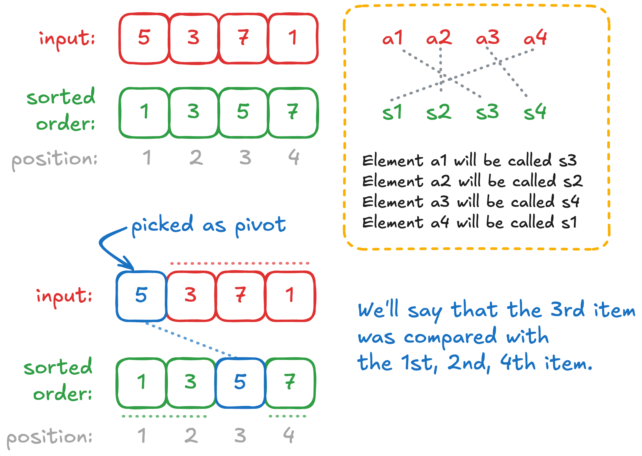
For example, if the input was $5,3,7,1$, if we pick the element $5$ as the pivot, we’re actually going to think of this as picking $a_1$ which happens to be $s_3$, so we’ll think of this as taking the $3^{rd}$ item as the pivot (instead of the $1^{st}$). There’s going to be a reason for this.

Let $C_{i,j}=1$ if during the run of the algorithm, $s_i$ was compared with $s_j$. So in the example above, $C_{3,1}=C_{3,2}=C_{3,4}=1$. Also being compared is a symmetric relation, so for example $C_{1,3}=C_{3,1}$. Otherwise, if $s_i,s_j$ are never compared, then $C_{i,j}=0$.

Let’s think about this a little bit. Let’s say we knew for a fact that $C_{2,3}=1$. What can we now say about the pivot selection? Remember the only comparisons happen due to the partitioning function, and swaps only happen when the comparisons trigger it. So either element $s_2$ or element $s_3$ was selected to be a pivot at some point in the execution of quicksort.

Bear in mind the moment something was selected as a pivot once, it will never be selected as a pivot again. Furthermore, a pivot actually partitions the array. E.g. if element $s_3$ was selected as a pivot first. Then we know that element $s_1$ and $s_4$ will never be compared again after that.

Okay, so what we want to say is:

$$C=\sum _{i=1}^{n-1}\sum _{j=i+1}^n{C}_{i,j}$$

literally counts the total number of comparisons made during quicksort. Because it literally iterates between all the distinct pairs $\{i,j\}$. Now:

$$\mathbb{E}[C]=\mathbb{E}\left[\sum _{i=1}^{n-1}\sum _{j=i+1}^n{C}_{i,j}\right]=\sum _{i=1}^{n-1}\sum _{j=i+1}^n\mathbb{E}[C_{i,j}]$$

And again, since $C_{i,j}$ is only either $0$ or $1$:

$$\mathbb{E}[C_{i,j}]=0\cdot \mathrm{Pr}[C_{i,j}=0]+1\cdot \mathrm{Pr}[C_{i,j}=1]=\mathrm{Pr}[C_{i,j}=1]$$

So combining with the above, we get:

$$\mathbb{E}[C]=\sum _{i=1}^{n-1}\sum _{j=i+1}^n\mathrm{Pr}[C_{i,j}=1]$$

Okay so again, what’s the probability that $\mathrm{Pr}[C_{i,j}=1]$? Well it’s the probability that $s_i$ and $s_j$ was compared. So let’s think about how that might happen.

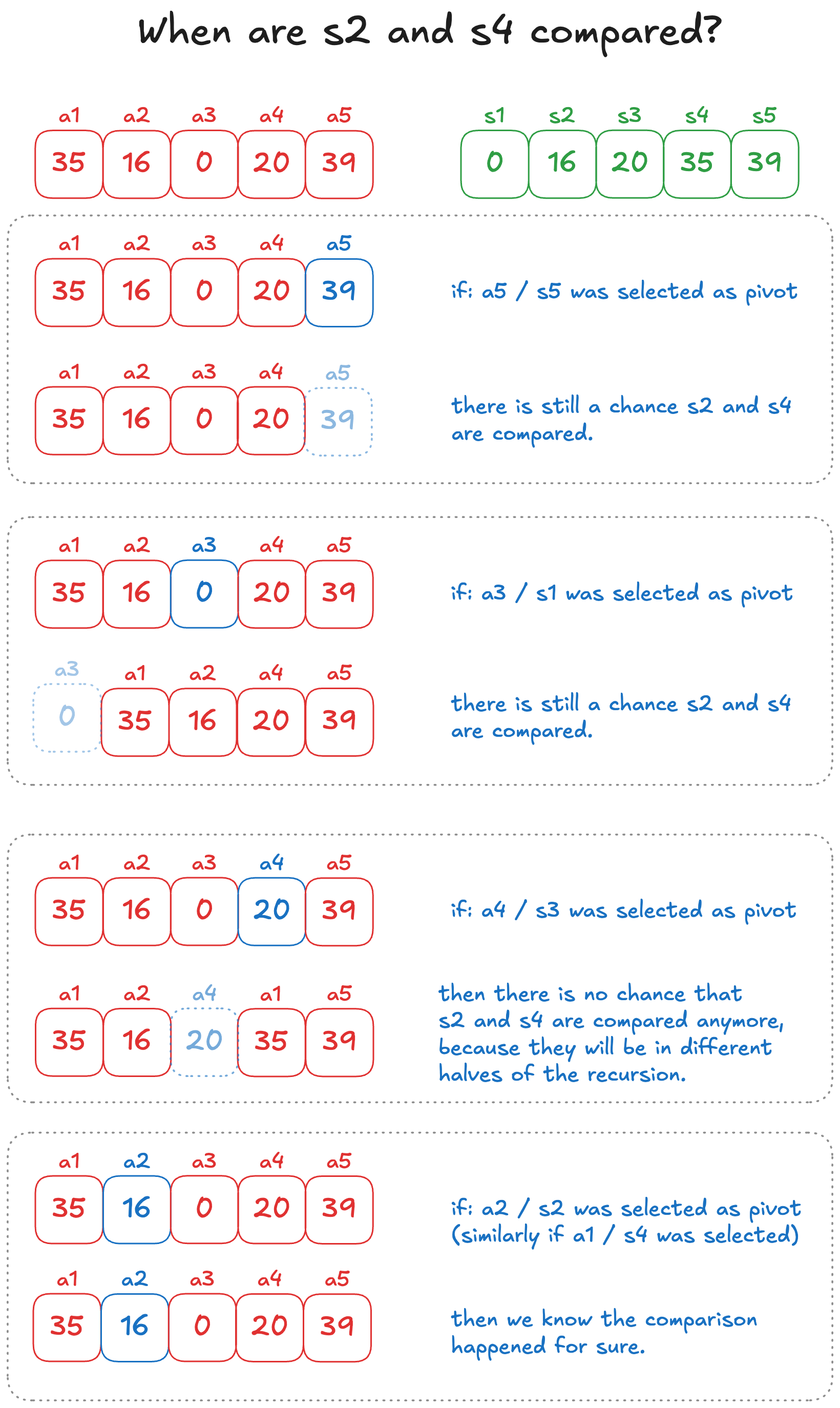
Here’s an example where the array (or sub-array) we wish to sort has 5 elements. For example if we care about whether $s_2$ and $s_4$ were compared, there’s actually $3$ possible cases:

1. Either at some point in the algorithm we picked element $s_1$ or $s_5$ as the pivot. In which case, it’s inconclusive as to whether or not $s_2$ or $s_4$ was taken.
2. Or at some point we picked $s_2$ or $s_4$ as the pivot. In which case we know for a fact they were compared.
3. Or at some point we picked $s_3$ was picked as the pivot. In which case we know for a fact that $s_2$ and $s_4$ will never be compared.

So in general:

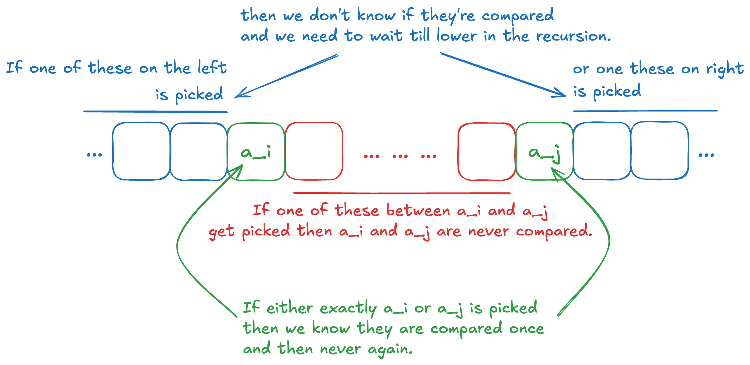
So for some two elements $s_i$ and $s_j$, first of all note we don’t care if anything before $a_i$ or after $a_j$ was chosen as pivots at any point in the execution. What we care about is in the sequence $a_i,a_{i+1},\dots ,a_{j-1},a_j$ was chosen as pivots. If $a_i$ or $a_j$ was chosen as a pivot, then $C_{i,j}=1$. Otherwise, one of $a_{i+1},\dots ,a_{j-1}$ was chosen. In which case, $C_{i,j}=0$.

Since pivots are chosen randomly, the probability that either $a_i$ or $a_j$ is chosen, is just $\frac{2}{j-i+1}$ because there are $2$ valid choices, and the are $j-i+1$ possible choices including elements from $a_i$ to $a_j$ (inclusive).

Now to finish it all off, we get that:

$$\begin{array}{rl}\mathbb{E}[C]& =\sum _{i=1}^{n-1}\sum _{j=i+1}^n\mathrm{Pr}[C_{i,j}=1]=\sum _{i=1}^{n-1}\sum _{j=i+1}^n\frac{2}{(j-i+1)}\\ & =\sum _{i=1}^{n-1}\sum _{k=2}^{n-i+1}\frac{2}{k}\\ & \le \sum _{i=1}^{n-1}\sum _{k=2}^n\frac{2}{k}\\ & \le \sum _{i=1}^{n-1}2(\ln (n)+O(1))\\ & \le 2\ln (n)+O(n)\end{array}$$

where on the first line we use the fact that we’re summing $\frac{2}{2}+\frac{2}{3}+\frac{2}{4}+\cdots +\frac{2}{n-i+1}$, so we might as well just change the variable to $k$ such that it ranges from $2$ to $n-i+1$ in the denominator. Then summing from $2$ to $n-i+1$ gives us fewer positive terms than if we just summed from $2$ to $n$, so the next line is an upper bound. Now, to see that it is $\ln (n)$, we use the following idea:

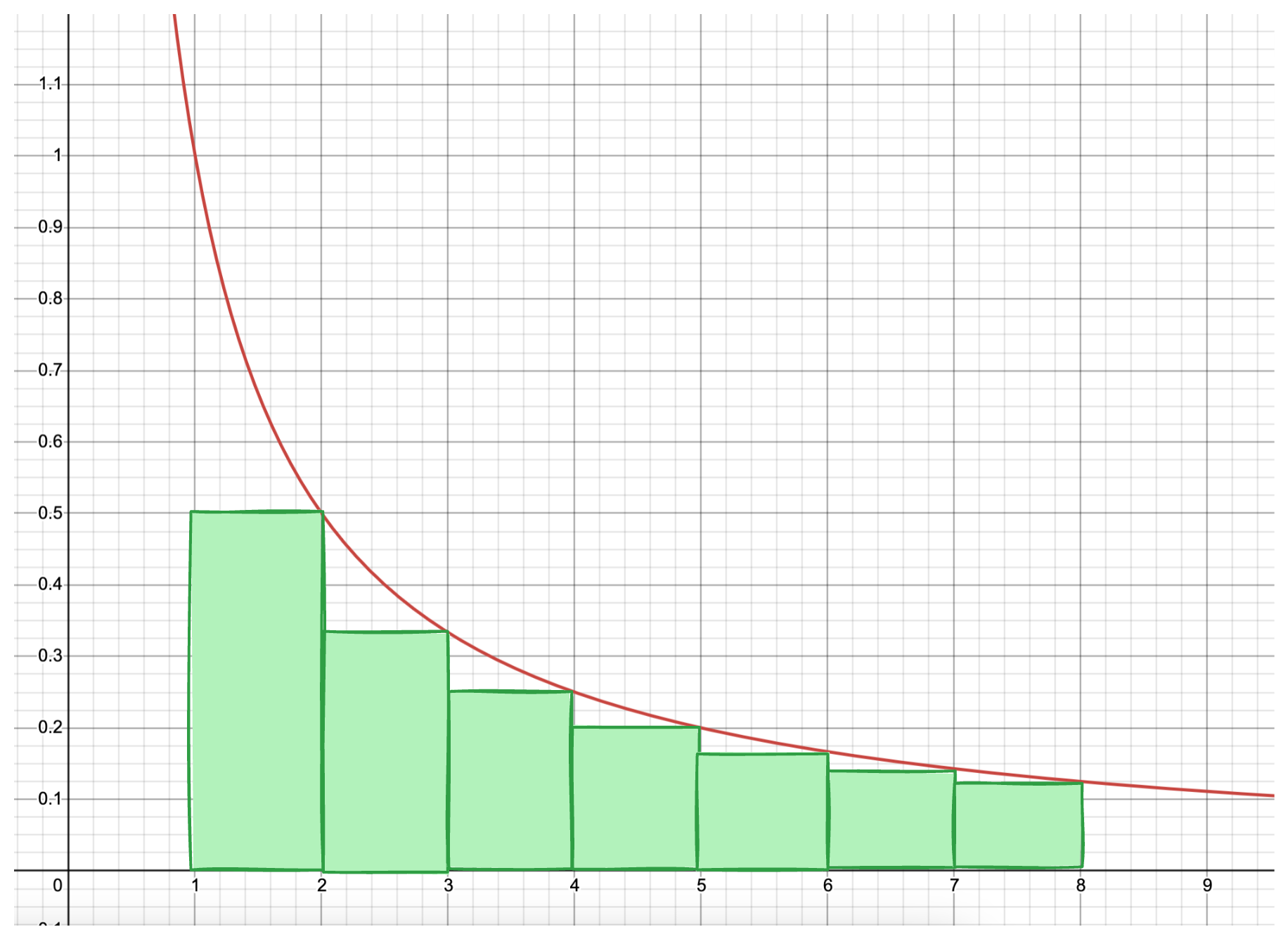
The red line plots the $y=\frac{1}{x}$ function. So the area under the curve is an over-approximation of adding $\frac{1}{i}$ for values $i$ from $1$ up to $x$. Thus the integral of $\frac{1}{x}$ from $x=2$ to $n$ is at most $\ln (n)$.

So! We’ve shown that the expected running time of randomised quicksort is $O(n\ln (n))$ (or $O(n\log (n))$, if you know that you can change bases between $\ln$ and ${\log }_2$ with a constant factor multiplication).